8. Working with Kaplan Meier
Investigate the prognostic value of a gene or a group of genes
8.1. Scope
- Use R2 to generate a Kaplan graph by “annotated parameter”. Use tracks or combine two tracks to assign the group separation of a specific dataset.
- R2 supports any type of survival data, such as overall survival and relapse free survival.
- Use the Kaplan Scan for a group of genes.
8.2. Step 1: Selecting the Kaplan Meier module
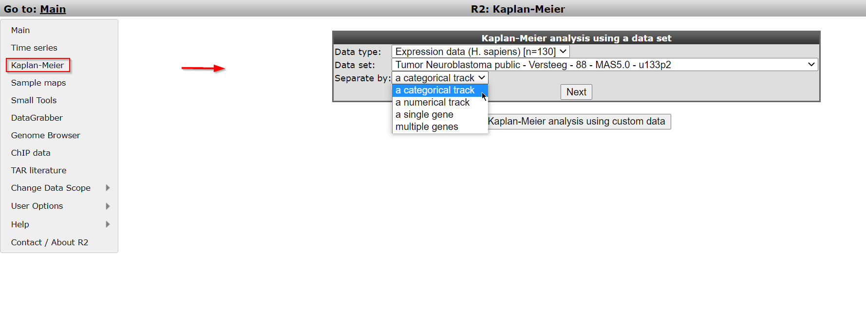
Logon the R2 homepage and select the option Kaplan Meier either in the left menu panel on the main screen or in field 3 at the type of analysis pull down menu. Using the Kaplan Meier module via the left menu directly shows from which datasets survival data is available.For this example, make sure that Data type is set to ‘Expression data (H. sapiens)[n=..’ and that Datat set is set to “Tumor Neuroblastoma public “ Versteeg “ 88”. From the dropdown of the setting Separate by choose the option ‘a categorical track’. Click Next.

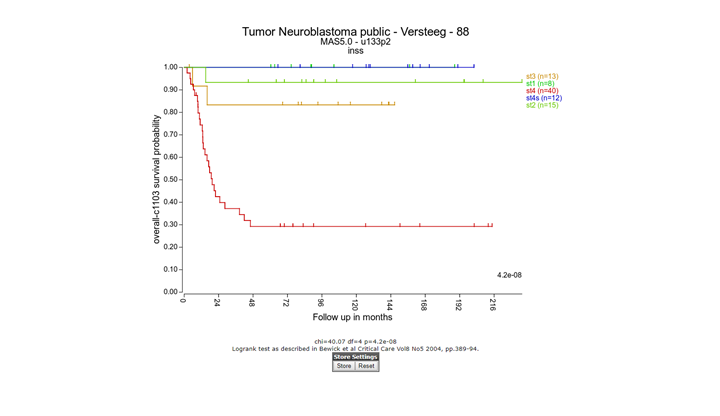
In the adjustable settings menu choose for Type of survival the value “overall-c1103”, select “track” at Separate by and select “inss (5 cat)” at the Track pull-down menu . Click “Next”. Note that stage st4s en st1 survival curves are overlapping which is in agreement with the clinical outcome of the INSS stages.
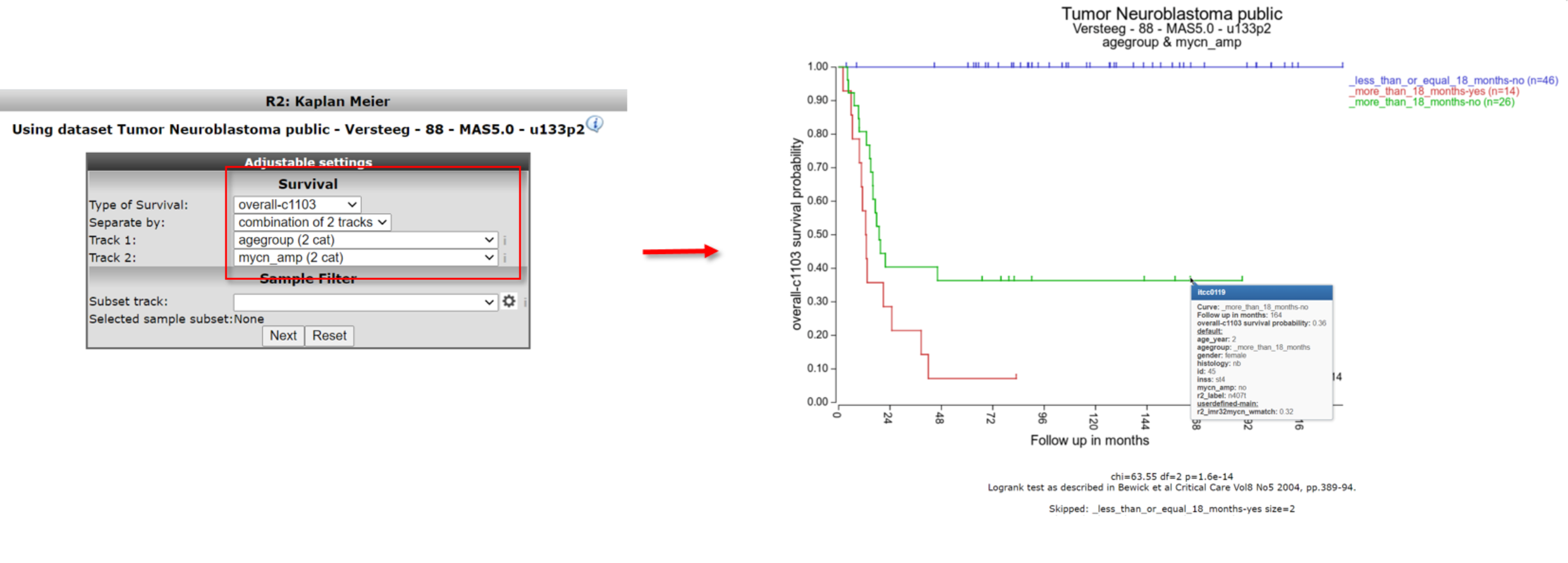
A handy feature of the R2 Kaplan module is the option to combine two tracks to generate subgroups for the Kaplan Meier analysis. Use the back-button from the browser and select at Separate by the option ‘combination of two tracks’. For example, choose for the first track ‘agegroup (2 cat)’ and for the second track ‘mycn_amp (2 cat)’. And click Next.

The combined track agegroup ( >18 year) and no mycn application results in intermediate survival probability. Note that there are 3 groups instead of “expected” 4 since there are no patients <= 18 year and a mycn amplification, in this cohort.
![]() Did you know that you can apply a filter to KaplanScan analyze a subgroup of patients for survival? In addition you can also adapt the graphical representation*
Did you know that you can apply a filter to KaplanScan analyze a subgroup of patients for survival? In addition you can also adapt the graphical representation*

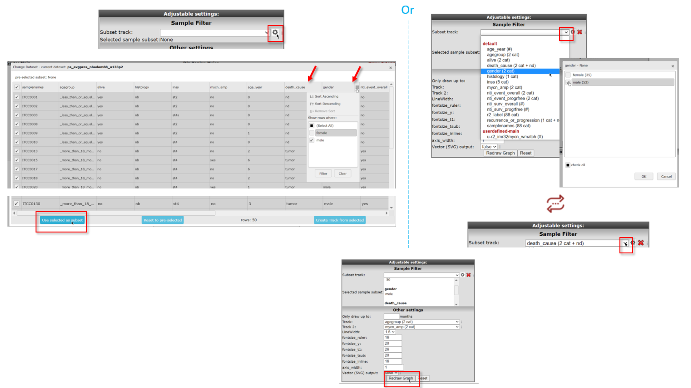
You can either use the annotation grid (left) or you can use the pull down (right) to select a subset of your samples by one or more tracks. If you click on the subscription of the picture above, the picture will open in large.
For the use of the grid, use the clog icon in the ‘Advanced settings box’ and hover your mouse over the side of the column of choice to show the filering options for that track. You can use the filtering options of multiple tracks to make a specific subset. Here we used gender to only select male samples (i.e. deselect female) and death_cause to select tumor and nd samples. A successful subset selection will be shown as a small message indicating the number of samples in the subset, the used track name and the number of groups/categories between brackets
If you instead want to make the subset selection with the pull-down of Subset track, click on the track by which you want to define the subset (in the example: gender). In the popup you need to check the box of your preferred subset(s) (here: male).If you want to further narrow down your selection with a different track, click on the same pull-down menu. Select the next track (here: death_cause) that you are interested in and in the popdown, check the preferred subset(s) from that track (here: tumor and nd).
Don’t forget to click on Redraw Graph after you made your final selection to redraw the Kaplan Meijer curve.
Nb. If you use the ‘back’ button in your webbroswer, then this selection will be lost and needs to be defined again.
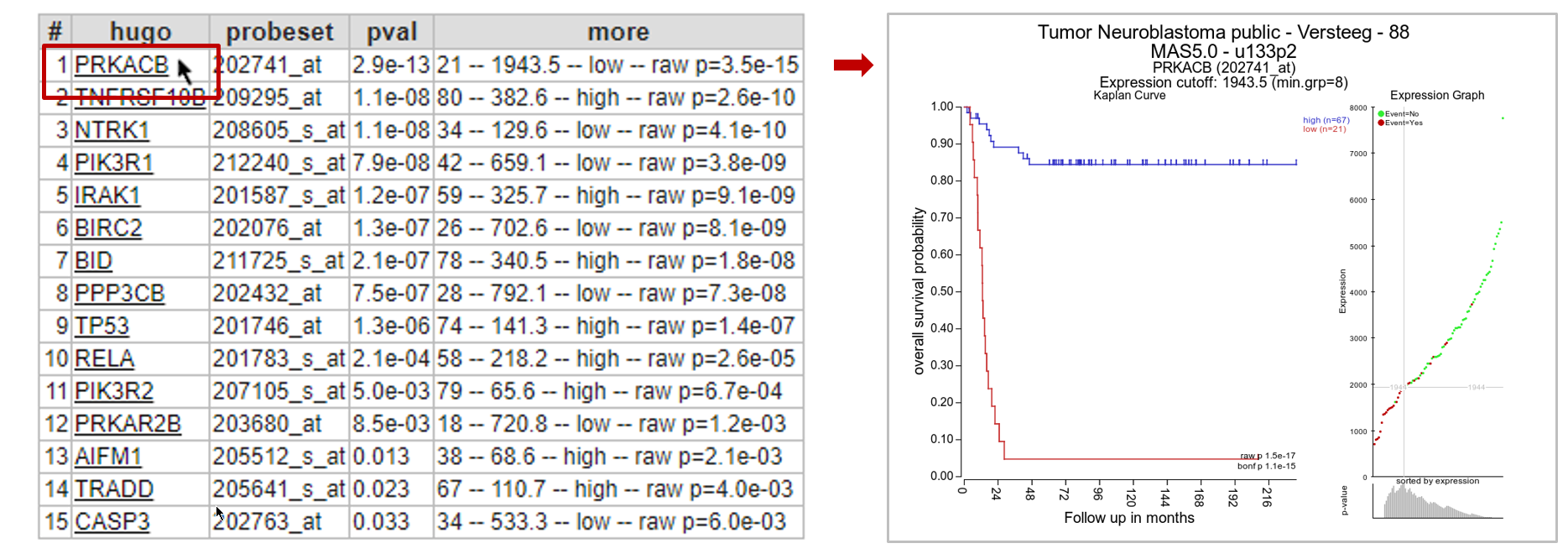
8.3. Step 2: Kaplan Meier by gene expression; the Kaplan Scan
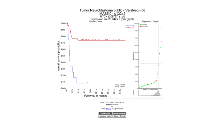
An often used feature of R2 is the Kaplan Scan (KaplanScan), where an optimum survival cut-off is established based on statistical testing instead of for example just taking the average or median. The Kaplan scanner separates the samples of a dataset into two groups based on the gene expression of one gene. In the order of expression, it will use every increasing expression value as a cutoff to create 2 groups and test the p-value in a logrank test. The highest value is then reported, accompanied by a Kaplan Meier picture. So in short, it will find the most significant expression cutoff for survival analysis. The best possible Kaplan Meier curve is based on the logrank test. However, R2 does also allow you to use median, average and more as a cutoff in assessing whether a gene of interest has the potential to separate patient survival. Of course, such analysis is only possible for datasets where survival data is present.
Select from the main screen either the left menu the Kaplan Meier option or in field 3 of the main menu, and choose Spearate by ‘a single gene’. Make sure that “Tumor Neuroblastoma public Versteeg 88” is selected with Data type ‘Expression data (H. sapiens)’, and click Next.
In the next screen fill in ‘mycn’ in the Search by Gene field and use the first reporter in the list of the dropdown that pospup. Leave the rest as is and click “Next”.
The Kaplan scan generates a Kaplan Meier Plot based on the most optimal mRNA cut-off expression level to discriminate between a good and bad prognosis cohort.
The determined separation in groups can be stored in a track and used in other analyes, click the “store as track” button
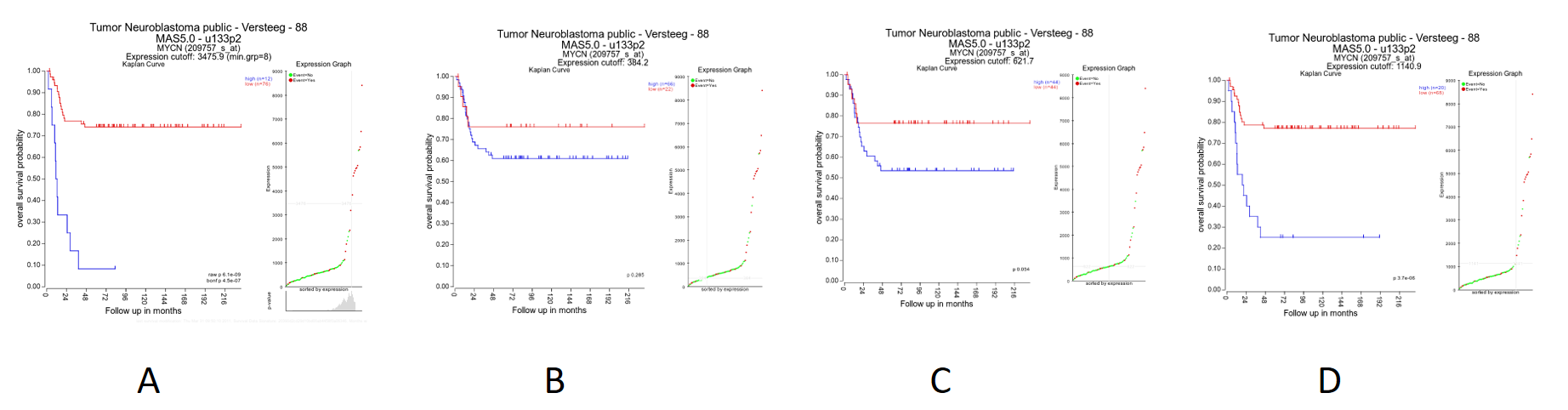
To illustrate that with the Kaplan Scan more significant biological subgroups can be found, adjust the cut-off mode to “median” in the settings menu and click Redraw Graph.

Figure 6: Kaplan plot with multiple cutoffs: A) Scan B) First Quartile C) Median D) Average
It is obvious that with the Kaplan Meier “scan modus” the sample grouping is much more significant compared to the median cut-off modus. Try to find out whether this is also the case with other cut-off modi.
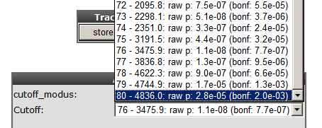
Next to the Kaplan plot in Figure 5, a small sub-plot is generated (underlined) which represents a graphical representation of the p-value plotted against the mRNA expression level values. In some cases it could be useful to change the p-value cut-off level and for this reason this graphical p-value plot (which is clickable) could be of help. Alternatively, you could use the “cutoff” field to regenerate a Kaplan curve with that separation.

8.4. Step 3: Kaplan scan for a group of genes
Instead of using the Kaplan Scan for a single gene you can also analyse a group of genes at the same time. Go back to the main page (”Go to Main” , upperleft corner), choose Kaplan-Meier from the left menu and choose Select by ‘multiple genes’ and click “Next”.
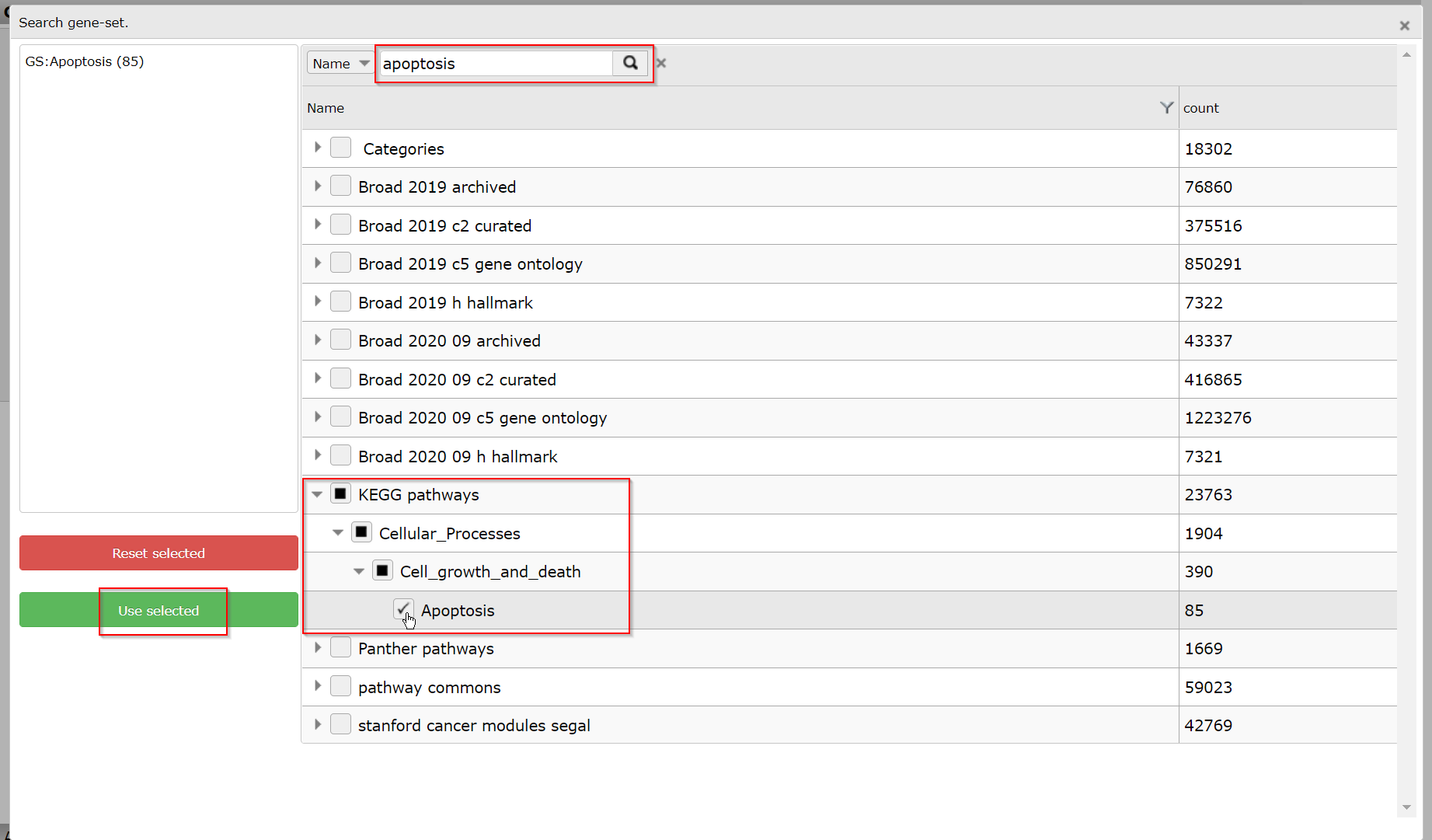
In this example search for a Gene set with the Search GS button. In the popup grid, type ‘apoptosis’ in the text field on top and click on the search button. In the adapted grid, open the KEGG pathways by a click on the arrow scroll and go on till you can check the KEGG ‘Apoptosis’ pathway. Click Use selected to go back to the menu, where the ‘GS: Apoptosis (85)’ geneset is now shown to be selected.

Leave the Type of survival at ‘overall-c1103’. In the statistics panel there are several filtering options possible, leave these options unchanged.
In the graphics section select “yes” at Draw heatmap and click Next.
In the next screen R2 has generated a list of the genes within the apoptosis pathway which have significant prognostic value. A heatmap for this list of genes is generated as well.

In Figure 8B, clicking on each gene name in the hugo column will result in a new screen or tab with the corresponding Kaplan plot.
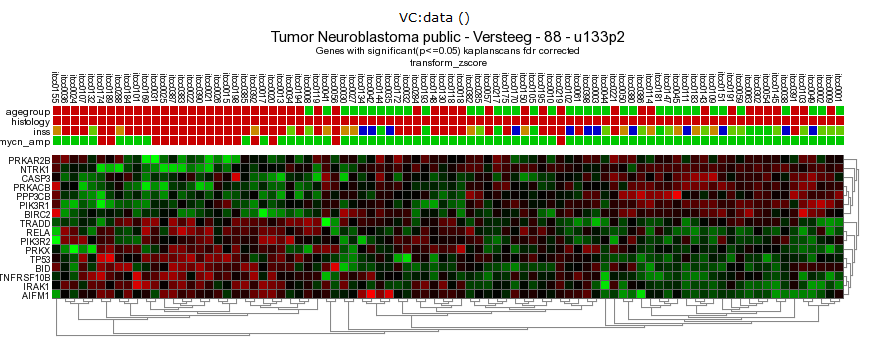
Figure 9: Heatmap of the significant prognostic list of genes.
In this case, the heatmap shows 2 or 3 possible biologically relevant clusters based on this set of genes. Clicking a spot in the heatmap will show directly the gene expression level for all samples via a new one-gene-view screen.
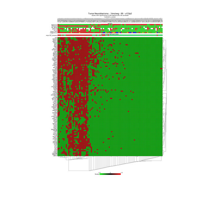
- To generate a binary heatmap based on the GOOD versus BAD prognoses, again go to the main page, click on Kaplan-Meier from the left menu, select ‘by multiple genes’ in the Separate by option, click next. This time don’t select anay gene set, but adapt in the Graphic Settings Draw a heatmap again to ‘yes’, choose in Heatmap data dropdown ‘good_bad (binary)’ and click Next.

Figure 10: Select binary heatmap.
Now the heatmap shows a clustering based on the GOOD vs BAD prognoses.
8.5. Step 4: Kaplan scan on your own cohort
It may happen that you would like to use the KaplanScan method on a dataset that is not available in R2. Especially for this reason we have made a user defined version within R2, where you can paste your cohort into R2 from e.g. a textfile and run the procedure. To initiate such a user defined Kaplan Scan, select the Kaplan Meier option again from the main page left menu, and click on the Kaplan-Meier analysis using custom data button underneath the panel.
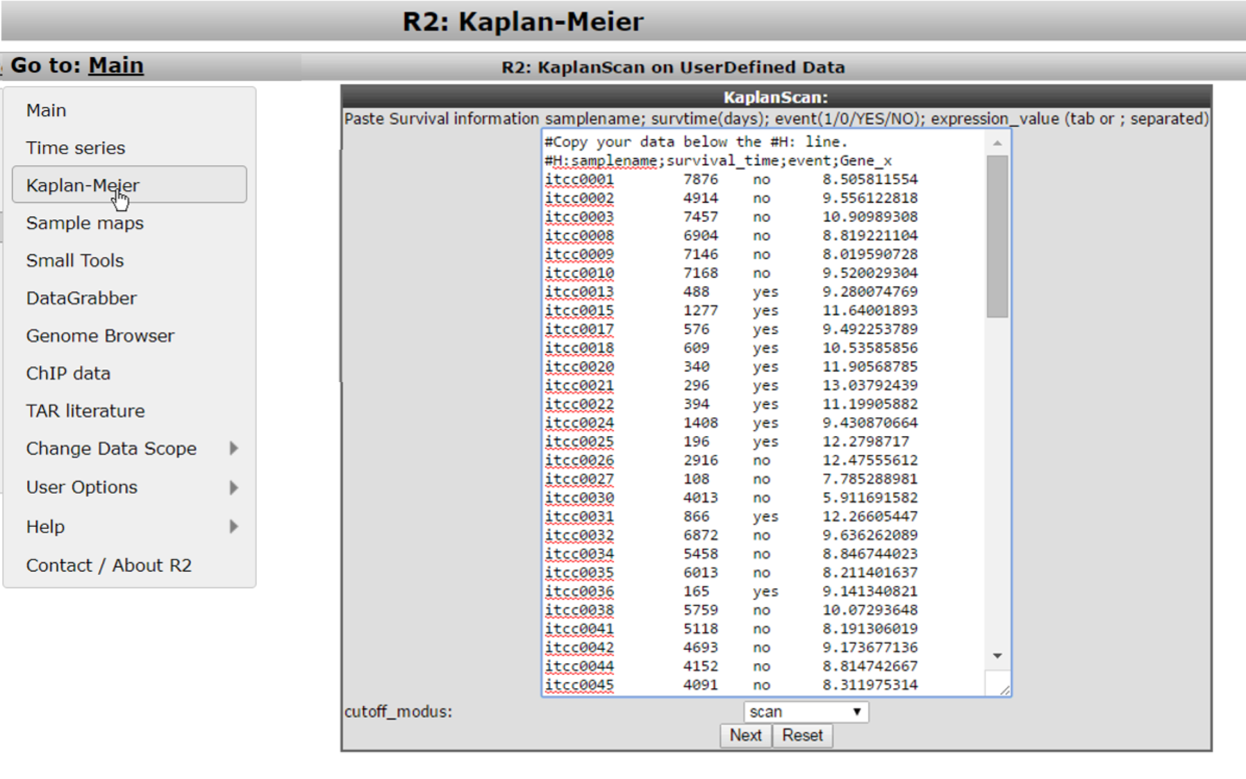
For the remaining steps to work as intended, we need to take into account a couple of things. You should prepare your data in the following four tab- or semicolon(;) separated columns.
- Column 1 contains a sample identifiers (without spaces)
- Column 2 contains the survival time in days (R2 will convert these)
- Column 3 contains the censoring information (event) and can be yes/no or 1/0
- Column 4 contains the expression value of the gene of interest for the kaplanscan
One can easily prepare this information in Microsoft Excel and paste the selected columns into the large white paste box. Do take care that we use “.” for decimal signs.
After you pasted the dataset information, you make the selection for the cutoff option and subsequently press next. R2 will now calculate the kaplan method that you selected and display the result in an interactive image.
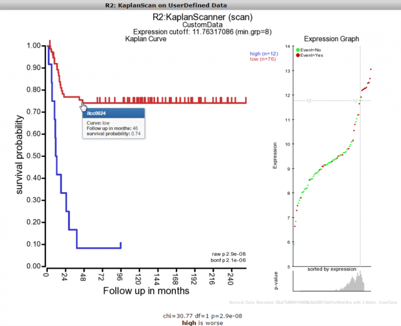
Once the image has been created, you are able to adapt various parameters to optimize appearance of your result.
![]() Did you know that the survival data used in your scan produces a unique signature?
Did you know that the survival data used in your scan produces a unique signature?
R2 will indicate within the image a checksum (MD5 sum) of all the survival information, which can be used to identify whether the same cohort information has been used in different scans that you may perform (this code should remain identical).
8.6. Final remarks / future directions
Everything described in this chapter can be performed in the R2: genomics analysis and visualization platform (http://r2platform.com or http://r2.amc.nl)
We hope that this tutorial has been helpful, the R2 support team.