15. Principle Components Analysis in R2
How to identify patterns or groups in your dataset using Principle Component Analysis.
15.1. Scope
- In this tutorial expression data of a set of Medulloblastoma tumors will be investigated for the existence of subgroups.
- Principle Component Analysis (PCA) will be used to analyze the tumor samples.
15.2. Step 1: Selecting data and modules
Make sure that the Single Dataset option is selected in field 1 of the step by step guide.
In field 2 locate and select the ‘Tumor Medulloblastoma PLoS One- Kool - 62 MAS5.0 -u133p2’ dataset by clicking ‘Change Dataset’
In field 3 select the ‘Principle Component Option’ option.
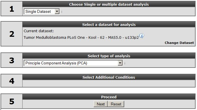
Click “next”
15.3. Step 2: Exploring the principle components
The next window displays a set of fields where specific settings of the clustering algorithm used can be set. Leave all the settings at their default and click “next”.
Click to plot the PCA result.
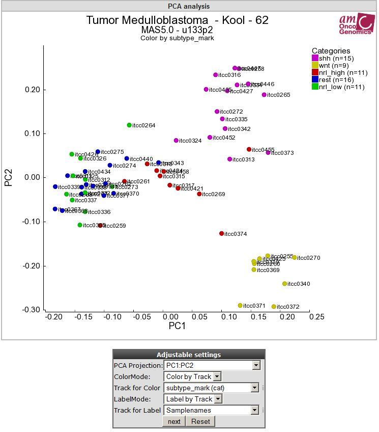
You now see a plot of the of the first 2 principle components. In the adjustable settings box, al the combinations principle components can be selected.
In the adjustable setting box select the all PCA-components option to view the several principle components combinations to investigate whether you can distinguish subgroups in your dataset.
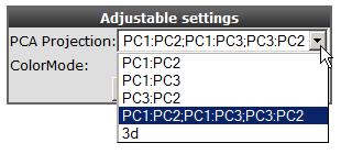
Figure 2: Adjusting PCA settings
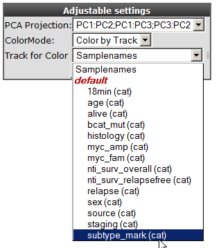
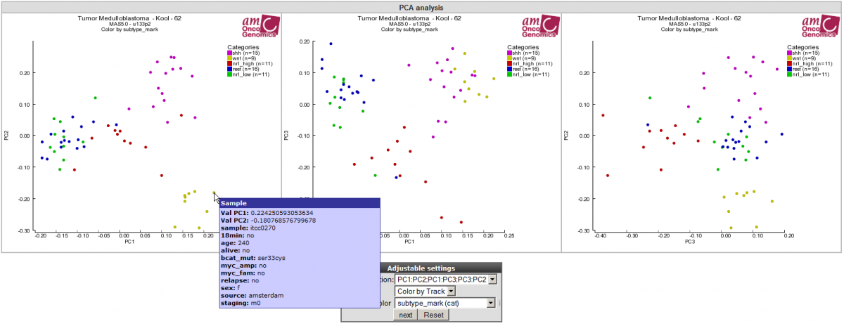
Figure 4: All 3 PCA-component combinations plotted in 2-dimensional space.
In this example the samples are colored by known groups and fitted with the PCA result. In Figure 4 a clear subgroup, the yellow wnt subgroup is revealed. Hovering over the data points provides the principle component vector #:values which are depicted, as well as additional sample information. This example illustrated that PCA is powerful tool aiding to find possible subgroups in your dataset of interest. Also note the variance reported on the axes.
5). Select in the adjustable settings box “Label by Track” under LabelMode. A “Track for Label” pulldown menu unfolds, here you select your track of interest e.g “Samplenames” and click next.

‘Figure 5: Samples are in annotated by track by usingLabelMode.
![]() Did you know that PCA clustering is a method that reduces data dimensionality?
Did you know that PCA clustering is a method that reduces data dimensionality?
Principle Component Analysis is a method that reduces data dimensionality by performing co-variance analysis between factors. PCA is especially suitable for datasets with many dimensions, such as a microarray experiment where the measurement of every single gene in a dataset can be considered a dimension. It is impossible to make a visual representation of the relation between genes and their conditions in multi-dimensional matrix. One way to make sense of data is to reduce dimensionality. Several techniques can be used for this purpose and PCA is one of them. The reduction of dimensions is archived by plotting points in a multidimensional space onto a space with fewer dimensions. The reduction is accomplished by identifying directions, so called principle components, that describe maximal variation in the data. These principle components can then be used as surrogates to represent each sample, making it possible to visually assess similarities and differences between samples and determine whether samples can be grouped. As the principle components are uncorrelated, they may represent different aspects of the samples and is therefore a powerful tool to identify subgroups in you dataset.
Each datapoint in the graph is now provided with a label annotation.
15.4. Step 3: Viewing clusters in 3D
A very nice feature of the R2 PCA module is the possibility to investigate your data in an interactive 3D-plotted graph. Most recent internet browsers support the 3D visualization.
![]() Did you know that browser settings might have to be adapted?
Did you know that browser settings might have to be adapted?
In Firefox in some cases it’s not possible to rotate the 3D graph in that case adjust the following setting in firefox. : type “about:config” in the URL box, search for webgl and Enable”webgl.force-enabled”: TRUE. The 3-D module also works with Chrome.
In the adjustable settings menu select the “3d” option and click “next”.
Click the cube and hold the left mouse button and rotate the picture in order to investigate whether there are any (more) subgroups that become visible.
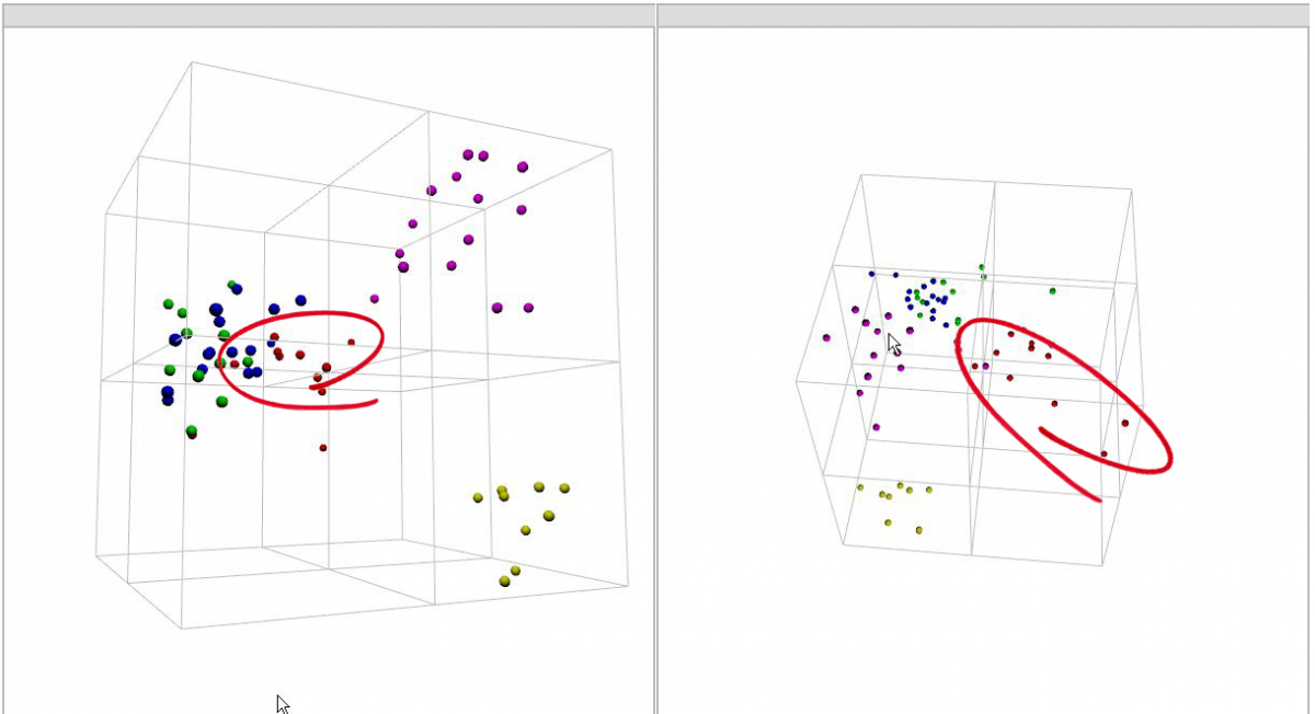
By rotating the graph more subgroups could be revealed as clearly shown in Figure 6.
15.5. Final remarks / future directions
The identification of medulloblastoma subtypes has been published here:
Kool M, Koster J, Bunt J, Hasselt NE, Lakeman A, van Sluis P, Troost D, Meeteren NS, Caron HN, Cloos J, Mrsic A, Ylstra B, Grajkowska W, Hartmann W, Pietsch T, Ellison D, Clifford SC, Versteeg R.; Integrated genomics identifies five medulloblastoma subtypes with distinct genetic profiles, pathway signatures and clinicopathological features. PLoS One. 2008 Aug 28;3(8):e3088.
Everything described in ths chapter can be performed in the R2: genomics analysis and visualization platform (http://r2platform.com / http://r2.amc.nl)
We hope that this tutorial has been helpful, the R2 support team.