22. Adapting R2 to your needs
Or how you can optimize R2 for your specific data analysis
22.1. Scope
- This tutorial describes the adaptable settings within R2. These are basically all items under the User Options menu-item. Through these you can personalize the use of R2
- First a couple of regular settings will be treated: changing colors, setting parameters
- Next we’ll delve into the practical adaptation of R2; uploading your dataset, adding your personal genesets ( categories), creating/exporting /uploading your own tracks and maintaining a user community
22.2. Step 1: Adapt your settings
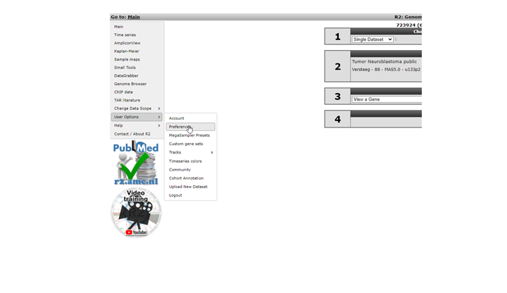
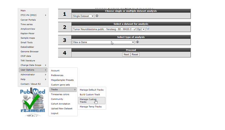
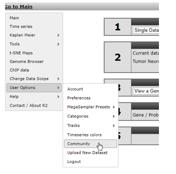
Personalizing R2 starts with selecting the ‘User Options’ menu item (Figure 1). When you hover over this item, you see a submenu. In ‘Account you can chose a different password or change your personal details.In ‘Preferences’ you can set some generic R2 analysis and visualization options, click on this item.
In the Preferences window several parameters for analyses in R2 can be adapted to your preferences. For most analyses these are set to appropriate values, but of course you want to set your favorite dataset here!
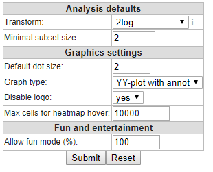
Figure 2: The User Defined Settings window: change settings at your own convenience
Next item in the User Options submenu (Figure 1) are the ‘Megasampler Presets’ . These are of relevance when you’ve built a specific Preset in an analysis Across Datasets ( see chapter: Multiple datasets overview with Megasampler).
The ‘Timeseries colors’ allows you to set the colors for the graphs of specific experiments in a series (Figure 3).
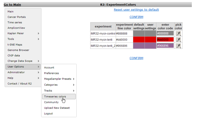
Figure 3: Setting timeseries colors
The other menu-items ‘Upload New Dataset’, ‘Categories’, ‘Tracks’ and ‘Communities’ will be discussed in steps 2 - 6 of this tutorial.
22.3. Step 2: How to add data to R2.
One of the most appreciated options of R2 is the possibility to add data to R2, be it your own dataset or/and publicly available data that matches your research interest. Due to several reasons, technical as security, it’s almost impossible to automate the process of adding data for standard users. In order to keep the database curated only R2 administrators can add data to R2.In order to do so, the data first has to be processed and uploaded. chapter 24 describes in detail how to prepare your data such that we can process it and upload the data to R2.
(r2-support@amsterdamumc.nl). If you would like to see a publicly accessible dataset in R2, then send an email to r2-support@amsterdamumc.nl with a link to the data, or in the case of a Gene Expression Omnibus dataset, the GSE**** identifier, matrixes in supplemental data and we will take care of the rest.
22.4. Step 3: Create your custom genesets
Another powerful functionality to adapt R2 analyses to your specific needs, is by defining gene sets or referend to in r2 as genecategories. Many analyses in R2 can be performed on a subset of genes ( see chapter 14 for a tutorial on performing gene set analysis). There are 3 main sources for gene sets. Firstly R2 harbors hundreds of predefined sets of genes (such as KEGG pathways or sets defined by the Broad Institute). Secondly, some analyses will result in gene lists, which R2 allows you to save on the fly such that they can be used for further analyses ( e.g. Toplister analysis) .Next to these two options, you can introduce your own gene sets of interest directly to R2 as well; Hover over the ‘ custom genesets’ sub-item and select the button ‘custom geneset editor’ (Figure 5).
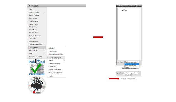
Figure 5: Geneset related menu-items; select Custom genesets to make your own.
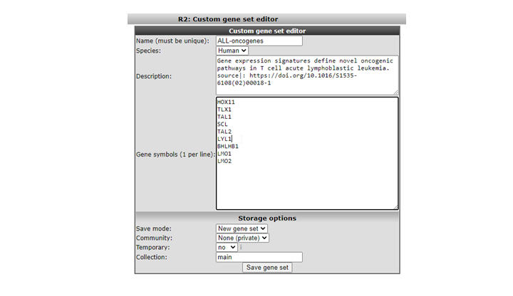
The ‘Custom Geneset editor’ window pops up (Figure 6). By default in this window you must provide a unique name for the set. The input box allows you to paste a list of genes to upload as a geneset for use in analyses in R2. In the example a set of genes, specific for ALL tumors are pasted. If you want this gene set to remain available for you, select in the community dropdown , “none” of select a community name for sharing the geneset. The concept “ commmunity” is descibed later in this tutorial. If you just want to store the set temporarily for 24 hours, choose ‘ yes’ in the temporary dropdown.Click “save geneset” to upload the set (Figure 6), you’ll receive a message when everything has succeeded. Your set of genes is now available as a geneset for all analyses within R2. Go back to the main page to see where you can use this set.
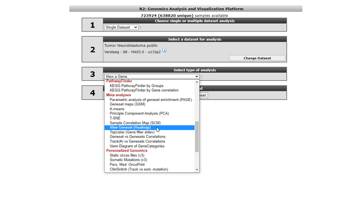
We’re going to lookup your geneset, an example is available in the Gene Set View. In the main menu in Field 3 select ‘View a Geneset (Heatmap)’ and click “next”( Figure 7)
In the GeneSetView your custom geneset is privately available for yourself for similar analyses as with any other public gene set present in R2. Select ‘My GeneCategories’ to choose from your categories. 6. If you saved your gene set temporarily, choose ‘My 24h GeneCategories’. And click Next and click Next again in the following window (Figure 9).
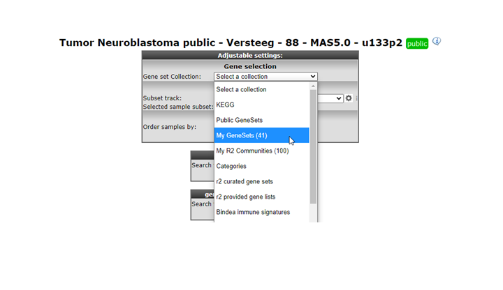
Figure 8: Selecting your genesets
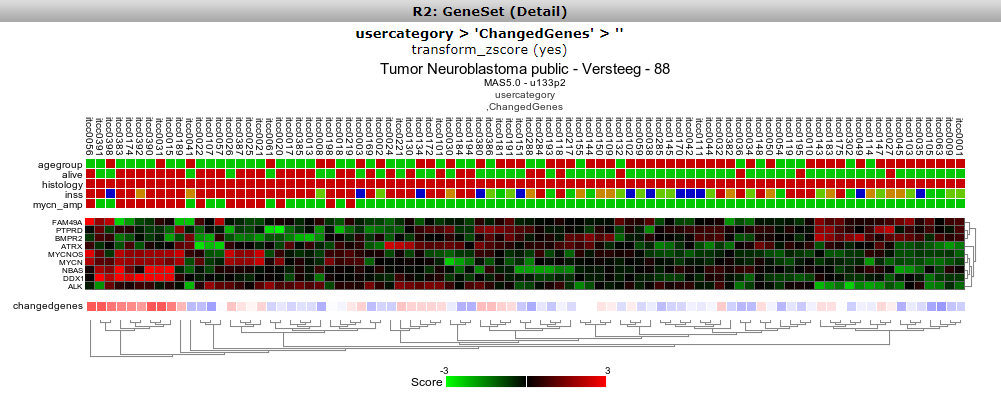
Now you can specify which gene set you want to view and how you want to the heatmap to be displayed. The geneset ‘ Changed Genes’ we just made above is available (Figure 9A), click on it. Also, in the Heatmap Options ‘color-scheme(v2a)’, select ‘green-black-red’, or any scheme that you prefer.For now we end here, later on we’ll see the geneset again in the context of Tracks.
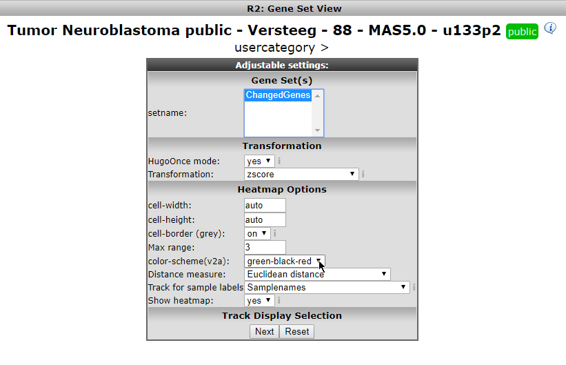
Figure 9 A: Your geneset is available.

We now return to the side menu of the R2 page to find out how we can manage the genesets we just built. From the ‘ User Options’ item in the menu, click Custom geneset. The custom geneset module allow you to organize you cuStom genesets , assigning the sets to a collection or delete custom sets.
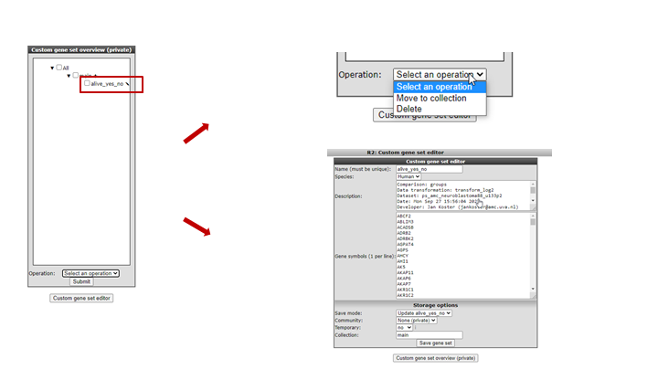
Figure 10: Adapting your genesets
Existing genesets can be adapted, deleted or moved to another collection. New genesets can be based on existing ones. As an example we’re going to update the genesets we just made. Click the ‘pencil’ icon next to the custom geneset in the custom geneset editor. In the next screen you can add or delete genes and provide background information and choose for the update of new geneset optipn in the pulldown menu.
22.5. Step 4: Tracks in R2: create your own data annotation
Another important feature in R2 that can be adapted to your needs are grouping variables, that we call “tracks” in R2. In R2, the samples can be annotated with sample characteristics, e.g clinical data or experimental characteristics. Each group of annotated data is called a “Track”. Tracks in R2 give you the opportunity to divide your samples in groups with e.g. different phenotypes for comparative or subgroup analysis. They also allow you to restrict your focus on only a part of the samples within a given dataset (when used in the ‘subset builder’). For some datasets the annotation that you need may be available already (from the default annotation that was added by the R2 team). For others you might want to add extra sample annotation for analysis such as combining already added tracks, or introduction of new information that you may possess. Tracks can be adapted in multiple ways:
- They can be uploaded with annotation files
- They can be created as a result of analyses within R2 and stored within the platform on the go
- Or you can create a so called Custom Track yourself within R2.
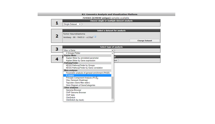
We’ll first start with an example of adding a track from the results of an analysis that is performed from within R2. We will illustrate this option using a K-means analysis. Such an analysis results in a division of the samples in two groups ( in the case of k=2. For more about this analysis see chapter 14). On the main page of R2 select the K-means analysis in Field 3 (Figure 11)
In the settings window for the K-means analysis (Figure 12) you can choose the geneset created above to cluster the current set of samples. In our case this is called ChangedGenes. Make sure that the number of draws is set to 10x10, click ‘next’
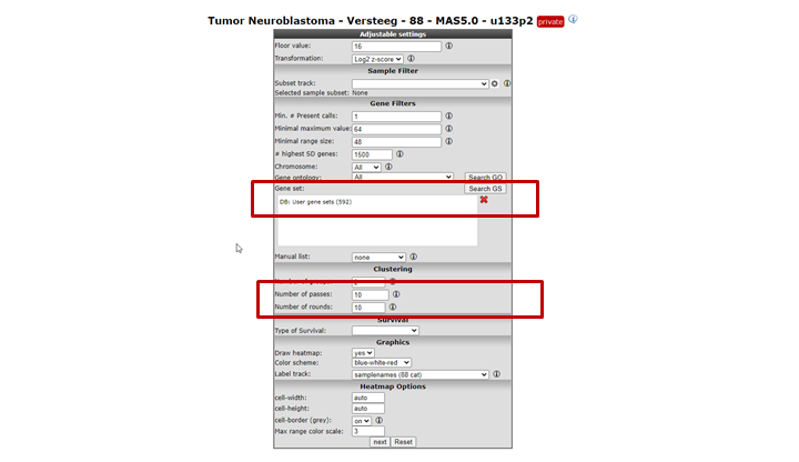
Figure 12: Settings for K-means; the Category built above is available for clustering
The resulting clustering in two groups might not be ultimately convincing (Figure 13, your result might look slightly different), but for our testing purposes this is alright. What is important is that the resulting groups can be stored as a new track, personal / available only to your account; click the button ‘store as a track’.
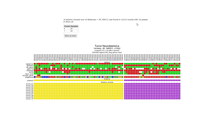
Figure 13: Clustering result of the Neuroblastoma dataset with a geneset built in the former steps
R2 now shows all samples as a long table with radio buttons indicating which group each sample belongs to. These can be adapted if you want to. Scroll down the window to find the fields that have to be set in order to store this as a track (Figure 14). You may want to change the group names into something more informative, and potentially also change the name to something you could easily relate to.
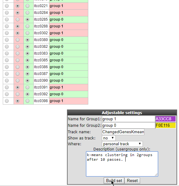
Figure 14: Storing the current groups as a Track for use in later analysis.
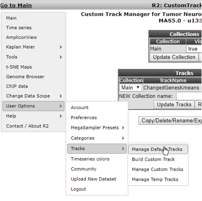
After optionally changing the parameters, you can click the Build set button to store the track. In the custom tracks manager we can adapt this track again. From the ‘User Options’ menu select ‘Manage Custom Tracks’ (Figure 15).

In the next screen keep the default selection, i.e. your current dataset. Tracks are, of course, defined based on a specific dataset; for each dataset you can store your own tracks. Click ‘Continue’.
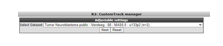
Figure 16: Tracks are defined per dataset; keep the current selection.
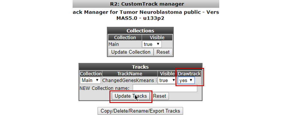
In the next screen you’re able to adapt the Track we just generated. Of interest in here is the option “Drawtrack”, which will result in the display of the information underneath the YY-plots.The tracks can also be assigned to collections to make large sets of tracks manageable. We leave the deletion of the track to the imagination of the reader.Now we’ll pay attention to the default tracks for this dataset. The track we just generated can be adapted from here. For a start set the Drawtrack propery to ‘yes’; we want to see this track in the graphs we create!
Select Manage Default Tracks from the ‘User Options’ > ‘Tracks’ sub-menu (Figure 18)

In the next screen the dataset has to be defined; keep the defaults and click Continue. You’ll end up in the Default Tracks Manager (Figure 19). Basically all annotation provided with this dataset is available as a track. Try out different things here.We’ll select additional annotations by changing their Drawtrack value to ‘yes’: age_year, gender and recurrence will be shown underneath graphs as well in further analyses.Also, we’ll set the Collection of age_year and agegroup to NEW. Next to NEW Collection name, we add a befitting name that defines this group of tracks. Here we typed ‘Age related’. Be sure to click the ‘Update Tracks’ button for these changes to take effect.
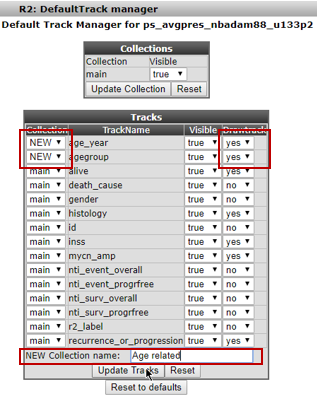
Figure 19 A: Selecting the default tracks for this dataset
When collections of tracks are used, these will show up conveniently as separate groups of tracks under the graph.
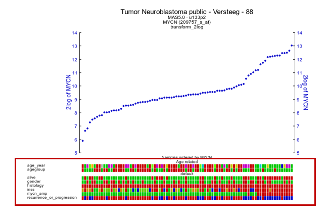
Figure 19 B: ‘Drawtracks’ makes tracks visible under the graph; group Tracks with ‘ Collections’
Use the ‘Reset’ button for Tracks or Collections in the Default Tracks Manager to undo either of the changes, or use the ‘Reset to defaults button’ to go back to the original dataset settings of tracks.
22.6. Step 5: Upload your own tracks
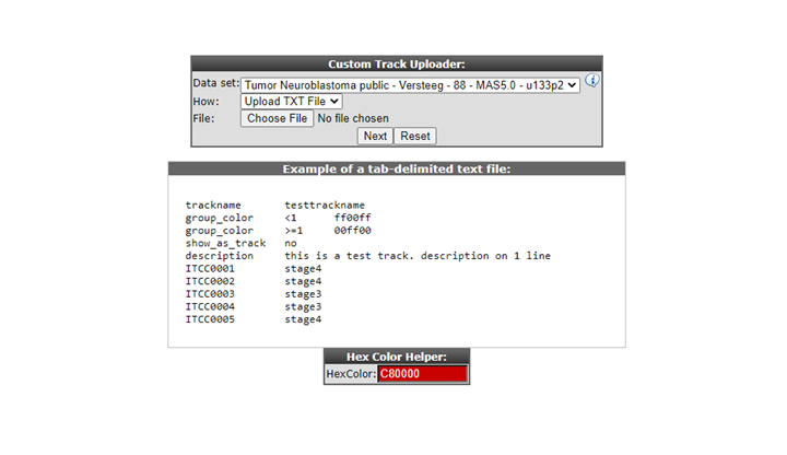
R2 also allows you to build your own tracks from scratch. You will be able to assign each sample to a group of your choice. To illustrate this select ‘User Options’ > ‘Tracks’ > ‘Build Custom Track’. The Custom Track window appears. R2 also provides the possibility to upload a custom track from a prefabricated text file. We will shortly show this route, which is also the most powerful one. Click ‘Upload or Paste a Track (txt file)’ (Figure 20).

In the Upload Custom Track window you can either select a tab delimited txt file built with a tool like Excel, or alternatively paste tab or semicolon delimited text in the input box. Either of these options provides R2 with the proper assignment of each sample to a specific value. Do note, that the internal identifiers (’samplenames’) that are used within R2, need to be provided here. Based on the values you provide in the second column, R2 creates the groups for you. You can create tracks with as many groups as you like. When described in a text file; for each sample a description can also be provided.
If you intend to create a track with a limited number of groups, an easier way is provided through the user interface. We will try that now: click the back button of your browser to return to Figure 20. By default the Custom Track Window (Figure 20) is set to build a track based on a defined number of groups. Underneath you can adjust the number of groups, now change the number to 3 groups and click the Submit button.
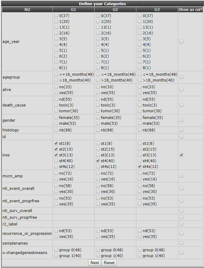
In the next window a convenient overview of all annotation parameters and their values is available, with check boxes to assign samples with specific annotation values to one of the three groups.In this example we divide the samples by their INSS classification values in 3 groups: the low grade(1,2,3) vs high grade(4) vs special (4s) tumor types. Tick the appropriate boxes in the appropriate group columns. It is also convenient to recapitulate the resulting groups in a separate column so tick that box also (Figure 25). In the inss row the stage 1-2-3 tumors are selected to form group 1, stage 4 forms group 2 and stage 4s group 3 in a new track.

Figure 22: Preselection to make new tracks from existing annotation.
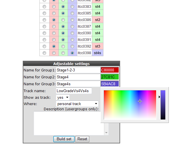
Click “next”, all samples appear in a table with check boxes to assign them individually to the appropriate group. Scroll down to adapt the visual characteristics of these groups. Names have been adapted, ‘show track’ is set to yes, the track is set to be stored as a personal track and colors per group have been adapted. Click ‘Build set’ to store the set, you’ll receive a message accordingly in the next window. Of course you now finally want to see all our track manipulation in an actual graph. Go to the R2 main page again, fill in a gene of choice (e.g. MYCN) in box 3 and click next twice to see how the data of a gene will be plotted using the new tracks.

Another frequently used approach is to make a track based on bins of gene expression values.To avoid labour intensive excel usage you can also use the expression treshhold option from the pulldown menu.Each time an expression level has been entered, a new box is generated for the next value.Of course, it is possible to change the names of the bins. Click next to tell R2 to draw the track, change the colors of the track bins and save the track.

Figure 24: Grouping samples for a track based on gene expression
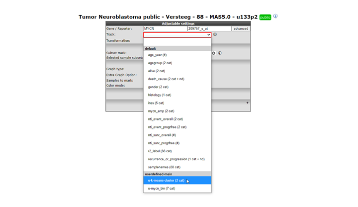
Select View a gene in groups in Field 3 of the main page, Click ‘next’. Type MYCN in the gene/reporter box, All the tracks created in the Custom Track manager are available for selection in the ‘userdefine’-main group of tracks, as a group separator choose inss stage, in this example we have switched off al the default tracks and selected the two custom tracks we have created.

Figure 25: Select the Track created in the Custom track manager; u-lowgradvs4vs4s
The expression of MYCN is plotted in the different groups of the inss stage (Figure 26). Extra Graph Option has been set to Track and Gene Sort. Note that the other track of mycn_bin groups the highest bin groups corresponds with the stage 4 group. Which also holds for the lower bin groups which are aligned with stage stage4s, stage 4s is known to have a better prognoses . There is also overlap with the custom created k-means generated tracks.
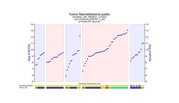
Figure 26: Tracks created are visualized underneath the graph
Another convenient option from the “custom track manager” is the export function which enables you to manipulate your tracks manually outside R2. This could be of use when your want to share tracks with other users or create new custom tracks. One reason you want to use the export function is to fix the ordering of your samples when generating a heatmap. Make sure you already have a personal custom track (not a temporary track, 24h). Select ‘Manage default Tracks’ from the User Options > Tracks menu (Figure 18) and click next. Here select the dataset of interest , only datasets which have a corresponding personalized track are represented in the pulldown menu. Click the “Copy/delete/rename/export Tracks” button. Here select the personal track , “export” operation and r2_track at “ export as”. Click execute” and download link with the track name can be loaded by clicking the right mouse button.
22.7. Step 6: Cooperate through R2: sharing tracks, creating communities
Cooperation is of great importance in scientific research. You probably want to share the tracks created above with other people in your group. For this reason R2 features the Communities. Communities are different from user groups, which is important to remember. User groups are granting a user access to datasets and their associated annotation. On the other hand, communities are a way by which any user can share grouping variables (tracks), lists of genes ( gene categories), megasampler presets or genome browser views with any (group of ) other R2 user(s). A user can generate multiple communities and invite other users to share such feature with.
Creating a community is done by clicking ‘Community’ in the ‘User Options’ menu (Figure 27).

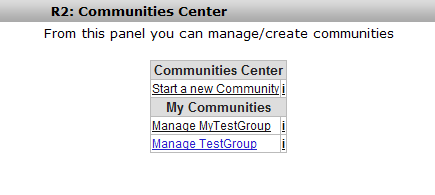
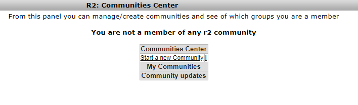
Since this will be the first time in the community section, there are no communities yet; click the ‘Start a new Community’ link (Figure 28).

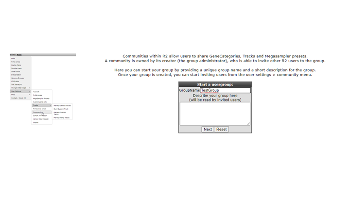
In the Community window a name has to be set and a short description for people invited as members for this group ( Figure 29). Through a community you can share your own Genesets,Tracks and Settings.

Figure 29: Setting the Community group name and description.
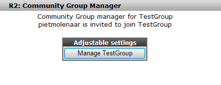
Click ‘Next’; you’ll be notified that the group has been created; return to the Communities Center by clicking the Community link again in the User Options menu (Figure 27). The TestGroup has been created (next to the already existing MyTestGroup for this user). Click the link to start adding users (Figure 30).
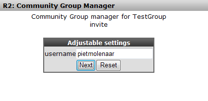
You have to add users by their R2 username; we’ll add user “pietmolenaar”. He’ll receive a message in the R2 startup page as soon as he logs on the next time. Click “next” to add the user.
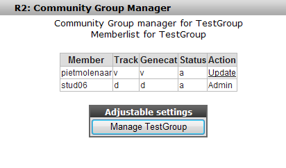
R2 returns with a message that the user has been invited, he or she has to accept your invitation first before he will see what you are sharing.

Figure 32: R2 return message; user is invited; but not yet visible
The perspective of the invited user after logon; he or she can accept the invitation (Figure 32).

When the invitation has been accepted the user is available in this community. When we add a custom geneset, track or preset the next time, it is possible to make this available to this community.
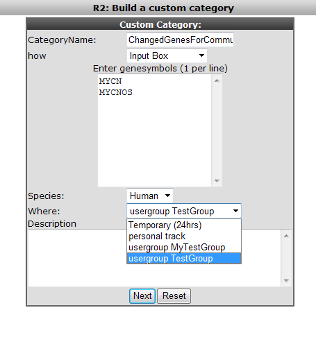
When a custom geneset is created there is now a possibility to make it available to a Community (Figure 39)
Managing the tracks, gene categories and megasampler presets is done in a similar way as has been shown in the user tracks and user categories at the beginning of this tutorial. pietmolenaar, as a member of this group, can manage the tracks that have been shared with him via his default track manager

Figure 35: As an example here the creation of a category and the assignment to a Community.
22.8. Final remarks / future directions
Some of these functionalities have been developed recently. If you run into any quirks or annoyances don’t hesitate to contact r2 support (r2-support@amsterdamumc.nl).
We hope that this tutorial has been helpful, the R2 support team.