13. Analysing Time Series
Search for up and-down regulated genes in a time series experiment
13.1. Scope
- Time series experiments, where a cell line is manipulated and followed over time, are analyzed and visualized in a separate section in R2. The actual analysis of any time series in R2 has been pre-calculated by the Affymetrix GCOS program. Within GCOS, every timepoint in a series has been compared to time-point zero. GCOS, makes use of the fact that every probe-set of an Affymetrix array is actually a measurement performed 11-16 times. These measurements are used as “independent” inputs to calculate a p-value. Due to the use of GCOS, the time series functionality is only available for the U133 type Affymetrix platforms. Of course, our advice would be to use biological replicates of all experiments.
- In most cases, time series experiments are performed by specific usergroups, whose data is often shielded from public assess. There are however also a few publicly available sets, to illustrate what this part of R2 can do. All the experiments performed on the same platform will most often be stored within a single set.
- Single gene expression levels can be visualized and list of regulated genes can be generated via a range of filtering methods. Please be aware that GCOS uses the probe information (contained within a probe set) from a single array to calculate p-values on. This is a controversial approach, but for many of the performed experiments the only way to obtain statistical values. If a timeseries experiment has been performed 3 or more times, then perhaps a better alternative would be to make use of the functionalities that are available for regular datasets.
- Use the time series module to investigate the expression level of a single gene.
- Use the time series module to generate a list of regulated genes.
- Use a list of regulated genes to analyze a dataset by using the geneset view.
- Use correlate with dataset to optimize your genecategory.
13.2. Step 1: Choosing the time series module and data
To view the expression pattern of a single gene from a time series experiment we make use of the “Time-series” module. Logon to R2 and select Time series in left menu panel of R2.
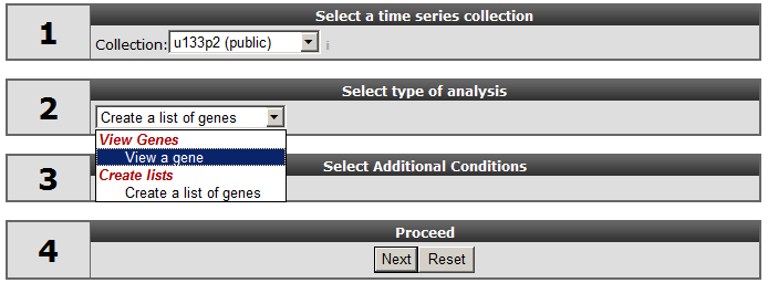
In field 1, select at collection “u133p2 (public)”. Here “collection” is indicated as a category of Time series experiments. For time series the analysis is limited to the Affymetrix Hu133A or Hu133plus arrays. The “Collection” field not only implies the platform type but may also include another subgroup , in this a case a publically available Times series data. Select “View a gene; in field 2, type HMOX1 in field 3*,* and click “next”.
In the next screen all the public available time series for the u133p platform R2 is hosting, is listed. In our example we make use of a Time series experiment published in Bioinformatics.”2010 Feb 15;26(4):456-63. In this Time series, the experiments are performed in triplo . The A549 Adenocarcinoma cellline is treated with TGF-beta and the expression levels where measured at several timepoints. In Figure 2 click on the (+) sign to unfold the Time-course experiments belonging to the A549 cellline and click “next”. In the adjustable settings menu, leave all the default settings and click “GO”.
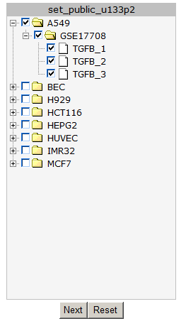
Figure 2: Timeseries selection screen.
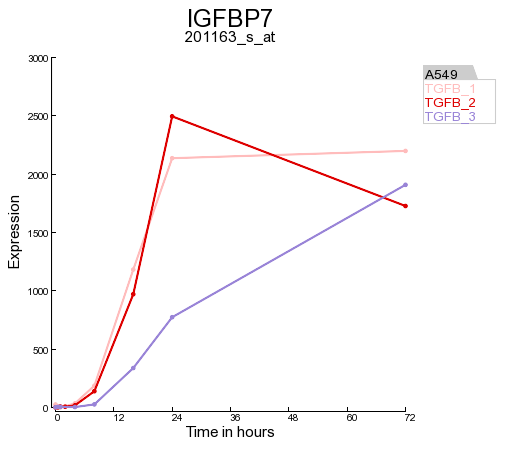
In Figure 3 the expression levels of the HMOX1 gene are represented in a triplicate Time course experiment after stimulation with TGF-beta. Clearly the HMOX1 gene is an early responder and is upregulated with a maximum at 4 hours. The HMOX1 gene is presented by the authors of the corresponding publication as one the upregulated genes after TGF-beta stimulation. It”s should be noted that a control experiment is missing in this experimental design. Hovering over the individual timepoint reveals additional information.
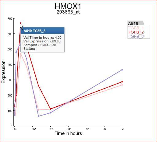
Figure 3: Expression levels of the HMOX1 gene during a time course experiment
Another gene the authors claim to be upregulated by TGF-beta is the BCL6 gene. In the same screen you can quickly generate a time series graph by providing the BCL6 gene in the right upper corner and click “Search Gene”.
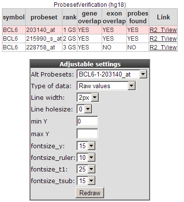
Figure 4: Probeset verification and Adjustable Settings.
The probeset verification table lists in the case of BCL6 the 3 probesets designed for the BCL6 gene. By default R2 will select the probeset with the highest average expression level. Clicking on the Tview link opens a separate application “Transcript view” to investigate the reporters in more detail. The Transcript view application is explained in tutorial 2 “one-gene-view”.
In the adjustable settings menu you can customize the Time series graph to your personal needs. Such as fontsize , Line width etc.
![]() Did you know that you can contact the R2-support team to add your Time-series experiments
Did you know that you can contact the R2-support team to add your Time-series experiments
*Your Time series experiments will be listed as a separate collection and for private analyses only. The R2-support team requires the CEL datafiles provided by your Microarray facility, to generate the result files. (see chapter 20) *
13.3. Step 2: Finding regulated genes in a time series experiment
Instead of looking at one single gene, you may most likely want to find novel up and-down regulated genes in your cell-line experiment. Go to the main screen and select in field 2 “Select type of analysis, “create a list of genes” and click “next”.
In the next screen select again all the A549 timeseries experiment and click “next”.
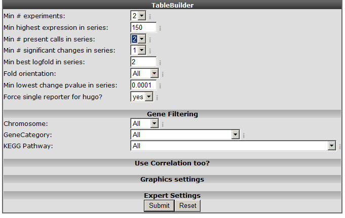
In following screen you can use the table builder to apply all kind of filtering options to find the novel regulated genes. Some of the options are already set.

Figure 5: The time series table builder.
An explanation of some of the options follows below: Min #experiments: Depending on your experimental design select in how many experiments your gene should be regulated according to your filter. Min highest expression in series: Set the minimal highest expression in at least one of the samples in your Time Series experiment. In this way the genes which are not expressed above a certain level (eg background) #:will be skipped. Min# present calls in series: The affymetrix MAS5.0 algorithm detects whether a gene is significantly detected and receive a “present call”. Min #significant change in series: Whenever the expression in a time series is significantly altered compared to time point 0, a “change” call is elevated. At least one change in expression level should be #:significant (meaning that you also would like to see those results where only in 1 time point a change is observed). Fold orientation: determine the orientation here. Up / Down / Both Minimal best fold in a series: Set a minimal logfold that has to occur within the series. Min lowest change pvalue in series: The MAS5 algorithm provides a p-value of the fold change, before a probeset is considered changed a minimal pvalue of 0.00025 should be met. Here you can set the pvalue to a more #:strict level. Force single reporter for hugo: It”s possible to analyse all probesets representing a single gene. As explained in another tutorial by default R2 will select the probeset with the highest average expression level. Select and set the options as depicted in Figure 5 and click “next”.
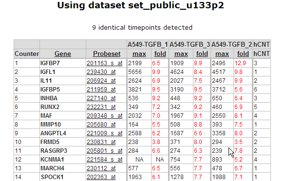
Figure 6: Up and down regulated genes table sorted on best fold change
In Figure 6 a part of the up and down regulated genes are shown, listing the fold change and highest expression level for each Time series experiment. Clicking on a probeset link generates a single gene time series plot as shown in Figure 7.
Clicking on the filter button will open the “adjustable settings” panel to re-adjust the selection options. Clicking on the Venn “diagram button re-direct to the automatically generated Venn Diagram representing the intersection of the genesets.


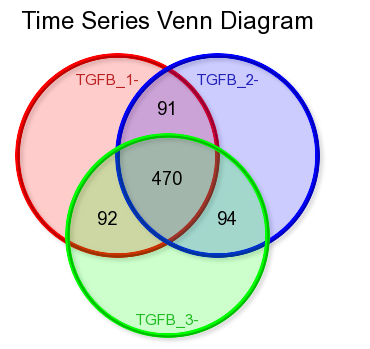
Figure 9: Time series Venn diagram
![]() *Did you know that Venn diagrams can be created directly from your genecategories of choice?
*Did you know that Venn diagrams can be created directly from your genecategories of choice?
In the ‘User Options’ menu section you can upload text files containing your lists of genes and store them as gene caterory. Repeating the procedure described above will produce the desired Venn diagrams.
13.4. Step 3: Using the regulated genes in further analyses
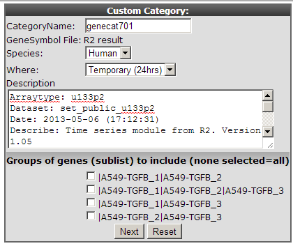
One of the strong points of R2 is that it supports directly further analyses with other modules and datasets stored in the database. Use the table of up and down-regulated genes of step2 to investigate if this list of genes can be of relevance in other datasets. In the left panel click “store results as gene category”. A new screen appears where you can enter an informative name for your genecategory and add a short description. The genecategory can be stored for 24 hours or stored permanently in your account, after which it is available each time you log in to R2. For now choose the Temporary option at “Where” and remember the name of the stored genecategory for the next step.

It has been published that the timecourse expression data from the cell experiment used in this example is linked to epithelial-mesenchymal transition (EMT) by TGF-beta induction. It”s also known that this process plays an important role in Breast cancer. We can use this generated genecategory to investigate whether this of any relevance or not.
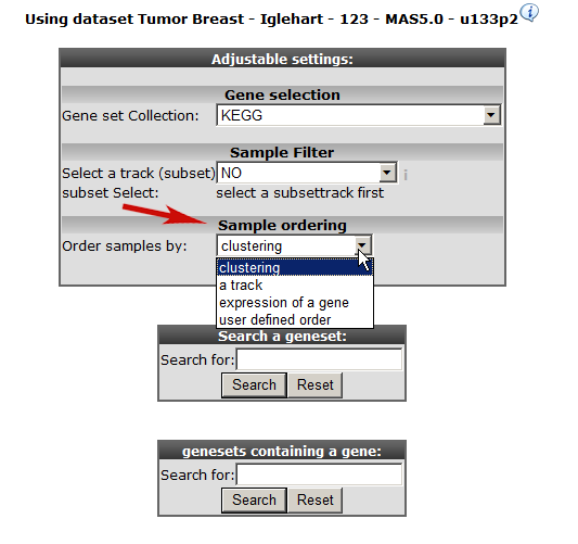
To keep the list of found genes for later usage, right click with the mouse on “Go to main” in the left upper corner and re-open the main screen of R2 in other tab/screen select at “change dataset” the following dataset . Tumor Breast - Iglehart - 123 - MAS5.0 - u133p2 . In field 3 select “View Geneset” at “Select type of analyses” and click “next”.

At “Gene set Collection” choose “ My 24h geneCategories” and select the generated “genecategory” from step 1. Instead of an unsupervised sample clustering you can also cluster samples within a track. Select at “Order samples” by “ ordering by track and click next.
Click next again.
Choose the temporary Genecategory generated via the Timeserie experiments, the track b-r_grade and click “next”.

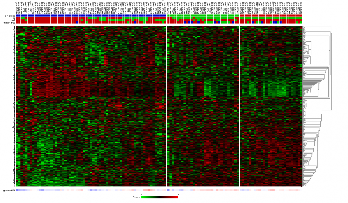
Figure 12: Heatmap of unsupervised clustering within a track of a selected geneset.
The samples are unsupervised hierarchically clustered within each group of the selected track and presented in a heatmap. The selected genecategory resulting from the timeserie experiment could be of clinical relevance since the clustering correlates with the Oestrogen Recepter track. At the bottom of the heatmap the z-scores of the selected genecategory is represented.
![]() Did you know that clicking a spot in the heatmap reveals more info
Did you know that clicking a spot in the heatmap reveals more info
Clicking on a heatmap rectangle generates a one-gene-view for the chosen gene in the dataset. Hovering over the heatmap rectangles reveals the sample information stored in the R2 database. Keep in mind that the hovering option is limited to 10000 cells, otherwise the graph generation consumes too much time. This limitation can be adapted in the ‘User Options’ menu item.
![]() Did you know that with “sample ordering” (Figure 11) you can manage the way the samples are clustered.
Did you know that with “sample ordering” (Figure 11) you can manage the way the samples are clustered.
By choosing “sample ordering “ by “track” , the unsupervised clustering of the samples is applied within the groups of a track. It is even possible to customize the way the samples are ordered by yourself (user defined order).
13.5. Step 4: Correlate with other datasets
The module “correlate” the results with dataset compares the resulting genelist with a dataset of interest. Go back to the screen/tab of the generated gene-list (see figure 6.) Clicking the correlate with dataset button in the left menu redirects to a new screen. Choose the Tumor Breast - Iglehart - 123 - MAS5.0 - u133p2 in field 2, in field 3 , choose “relate to differential expression” and click next.
Choose “er” at select a track and click “next”.
In de background R2 generates a list of genes based on the module “Find differential expression between groups” and presents the overlay of the results with the list generated in the “ time series module”.

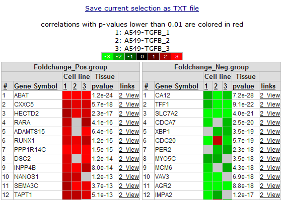
In Figure 14 the overlap is presented between the result from the “ time series” module and the “ relate to differential expression” option. The list of genes is sub-divided in a positive and a negative correlation list of genes. Clicking the “2-view” link opens a new screen with a combined graph of a one-geneview and the time series experiment.
13.6. Step 5: In a K-means analysis
Instead view a “ geneset, you can also choose perform a “K-means” clustering based on your stored genecategory described in the steps “ above”. Go to the main menu, select “K-means” at “ Select type of analysis” and click “next”.
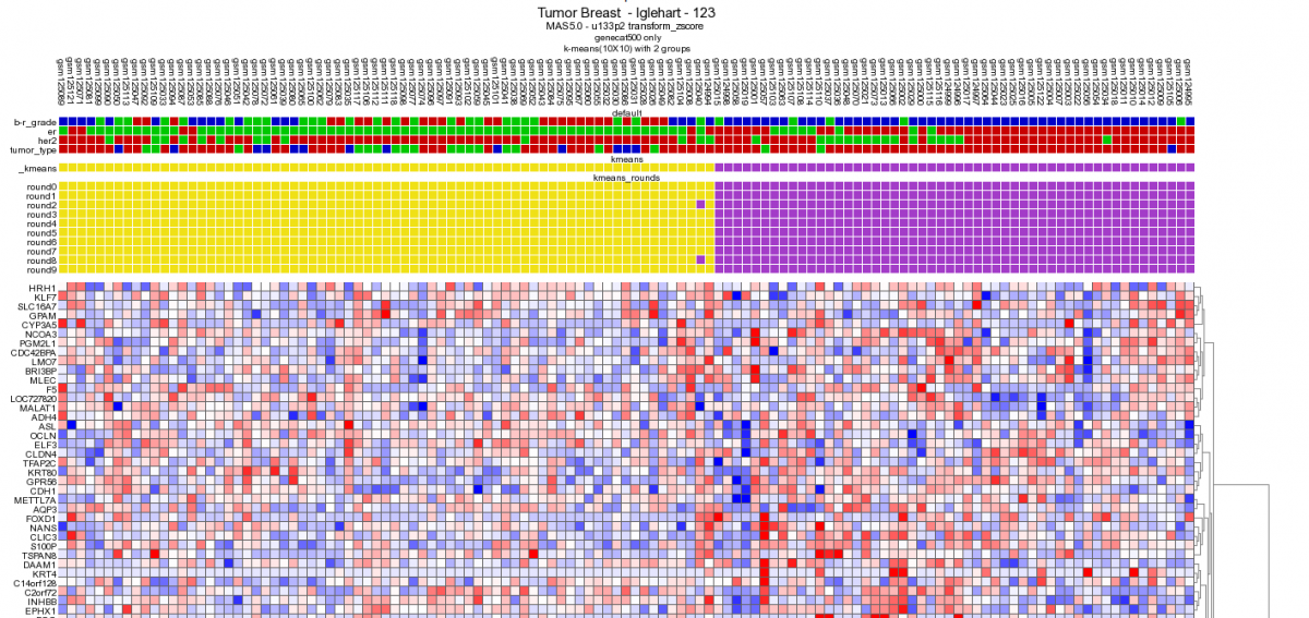
In the “Adjustable settings” panel leave most of the default settings but make sure that you select the already stored “Genecategory” at the clustering section select ‘10x10” at “numbers of draw” and click “next”.

Figure 13: 10x10 Heatmap with the same dataset and gene category as depicted in Figure 9.
Performing a 10x10 K-means clustering via de main menu supports the potential clinical relevance of the genecategory extracted from the timeserie experiment. The K-means cluster module is discussed in more detail in tutorial 10.
![]() Did you know that you can store the K-means generated track and use this track every time you log in to R2.
Did you know that you can store the K-means generated track and use this track every time you log in to R2.
You can use this track for further analysis with a custom made track for example by using the “find differential expression between groups”. This approach explained in more detail in tutorials : Differential Expression Of Gene Between Groups and “Adapting R2 to your needs”
13.7. Final remarks / future directions
We hope that this tutorial has been helpful, the R2 support team.